Port Tube Comparisons

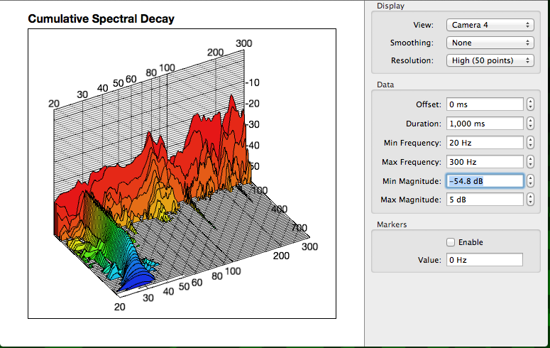
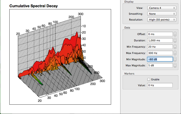
A port tube can extend the low-end response of a speaker beyond the lowest frequencies that can be produced by the woofer at an adequate volume. However, one of the drawbacks is that it takes time for the port tube resonance to die out. The best way to represent this is with a waterfall plot.

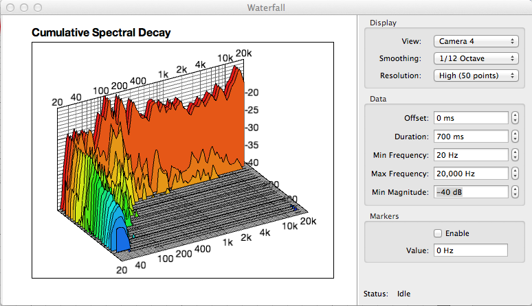
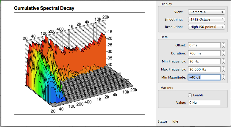
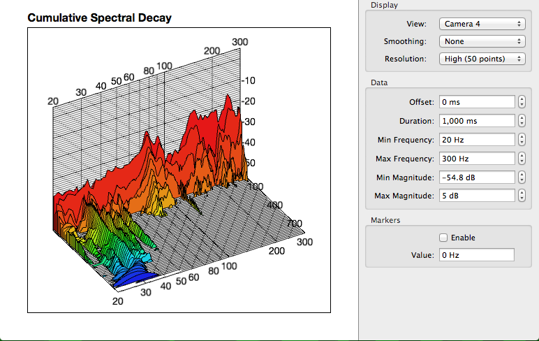
This shows the amplitude of all the frequencies decaying in time. The longest resonance is near the same frequency as the port tube. And when we plug the port tube with a towel…

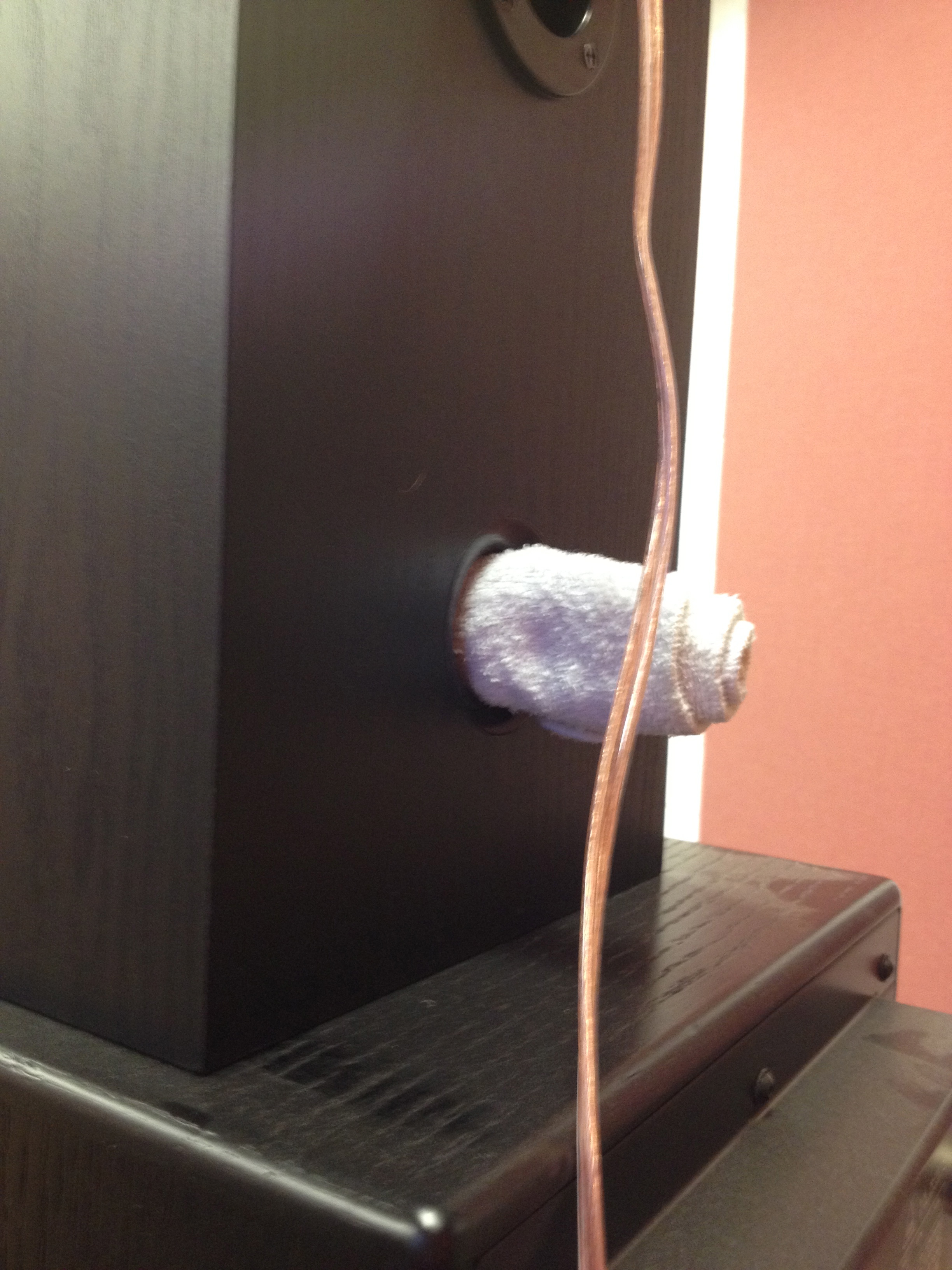
…. We can see that the resonance of the tube dies much more quickly.

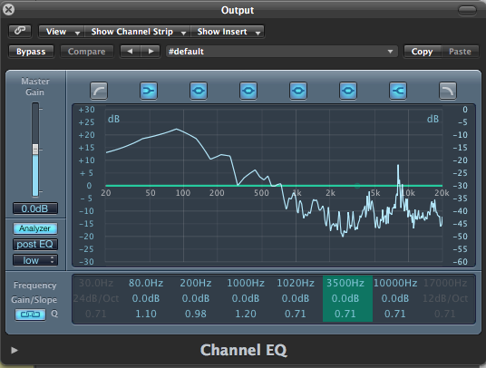
Subjectively, I want to hear more bass when I listen to the BR-1s, my speaker amplifier has a basic EQ, and the speakers sound more “flat” to me when I turn up the bass on the amp.

I find it interesting that what sounds “flat,” and subjectively pleasing to me is actually far from an ideal flat response.

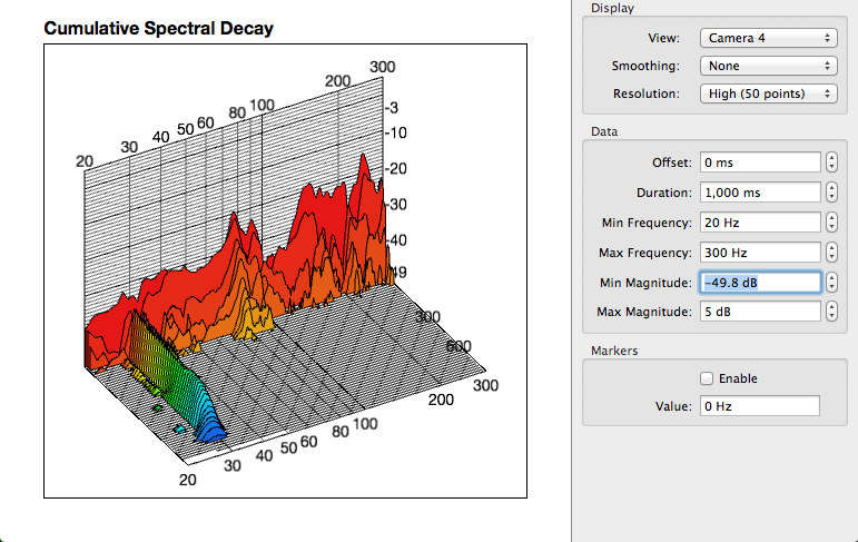
In order to better understand that data from the previous measurements, I also took some measurements at my apartment.

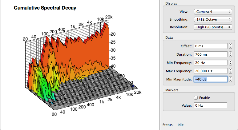
PORT NOT PLUGGED

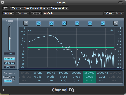
PORT PLUGGED

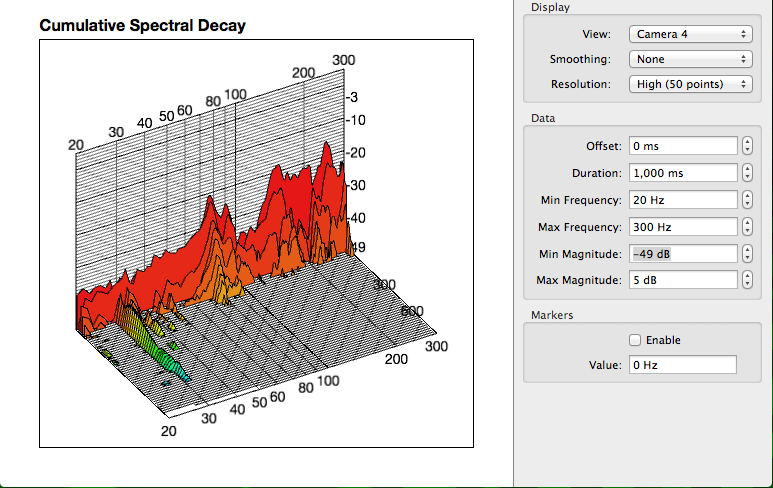
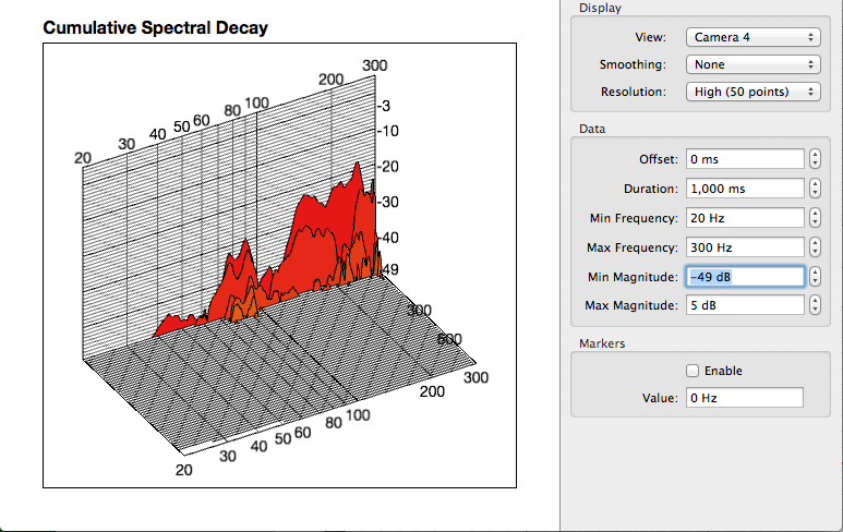
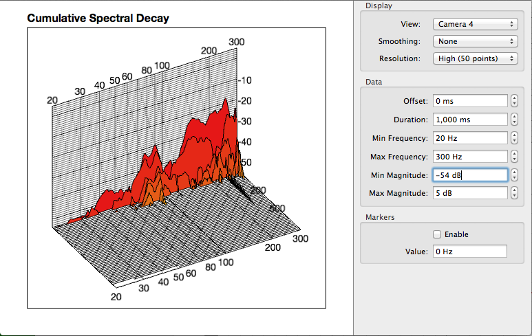
The graphs above show how the minimum value of the amplitude axis can greatly affect how the graph is interpreted. I tried to have the minimum value of the amplitude axis just slightly above the noise floor, which was at about -40dB.

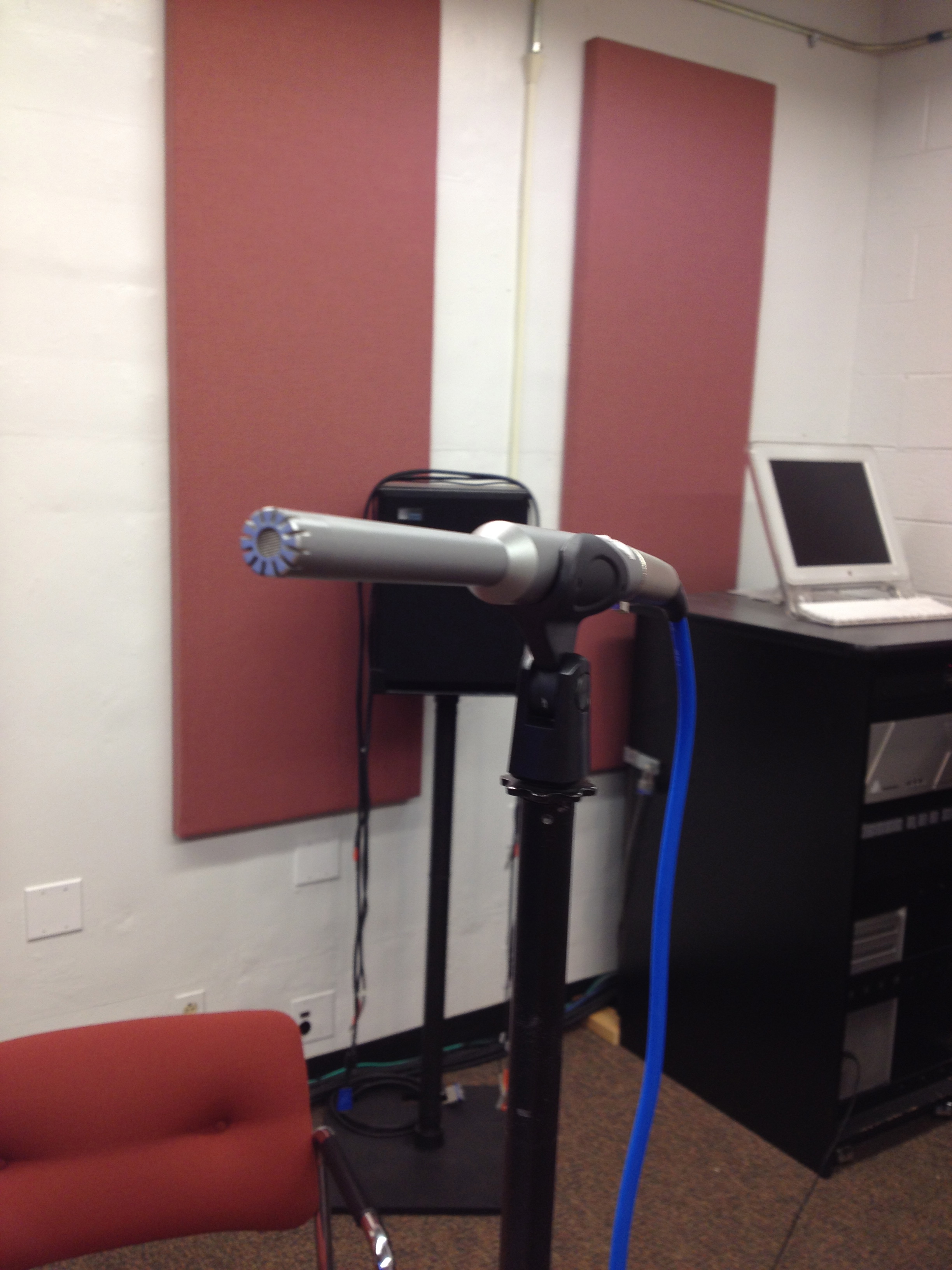
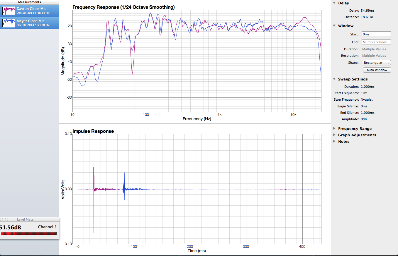
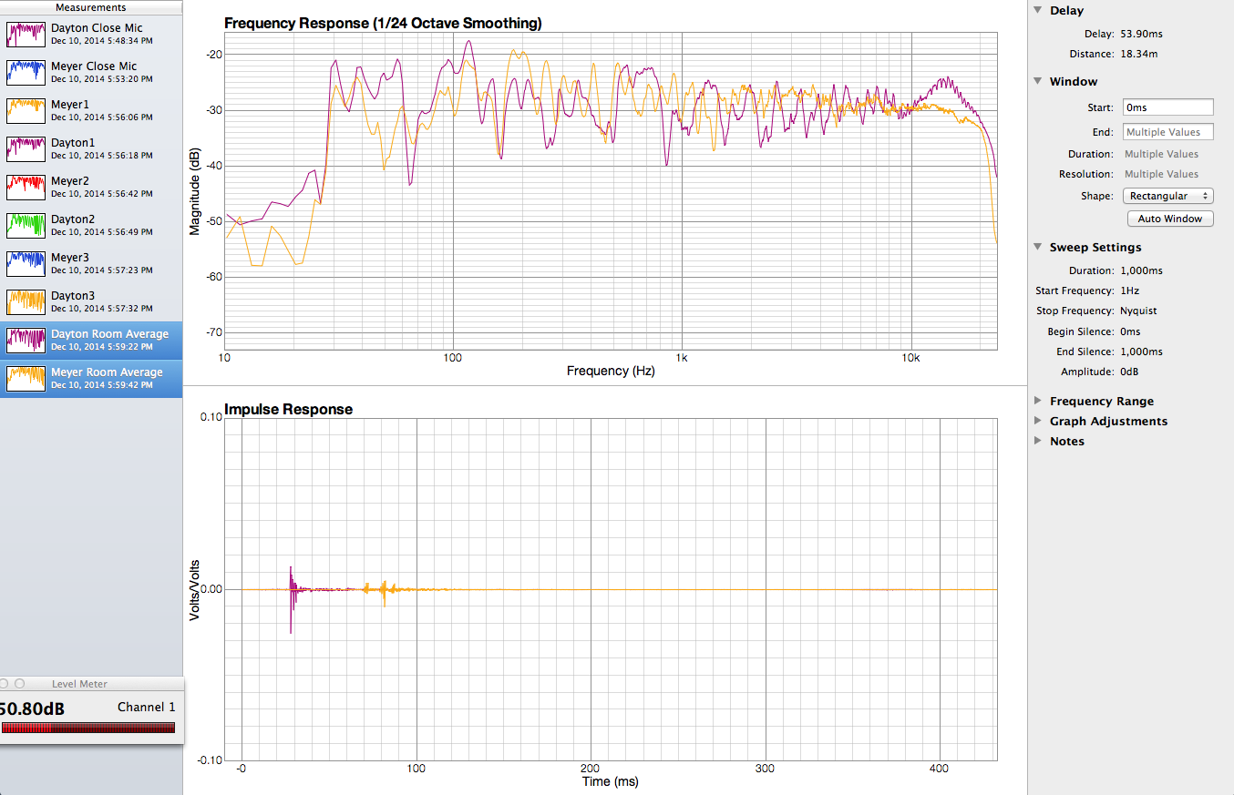
I also took measurements at my apartment with my Presonus M7 condenser microphone.

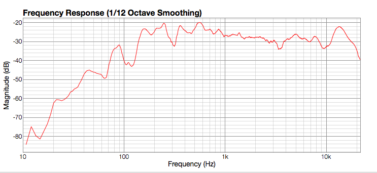
The Dayton Audio measurement microphone was clearly a good choice as the Presonus microphone leaves out a lot of the bass information.

BR-1 Comparison

It is difficult to measure the frequency response of speakers because microphones do not have a flat frequency response, and the resonate frequencies of a room make some frequencies louder than others. However, if we keep these variables consistent, we can learn about the performance of a pair of speakers by comparing them with other monitors using the same room and the same microphone.

The image above shows the frequency response of my BR-1and a Meyer Sound speaker which I believe was an HD 1. These measurements were made with the program Fuzz Measure, the Dayton Audio EMM 6 microphone, and my Presonus Audiobox audio interface.

The most noticeable difference between the two speakers is the peak between 10kHz and 20kHz in the BR-1s and the deep trough between 60 and 70 Hz.

Here are the frequency response graphs for the individual drivers given in the manual.

.

The stark differences suggest that my measurements were greatly influenced by the room modes. To try to compensate for this, I took measurements from many different locations around the room and averaged them.

The effects are noticeably reduced, and with a high enough sample size, could become negligible. However, it should also be noted that the resonant frequency of the port tube is 43 Hz– one of the peaks both graphs.

Crossover Circuit Measurements

I decided to try to do some of my own measurements on the BR-1 kit I build so I headed out to the lab.

I sent a sinusoidal signal from the function generator to both the oscilloscope and to my speaker.

I then measured the voltage over the woofer, and then over the tweeter while changing the frequency of the input.

I recorded the data from the oscilloscope.

Using Excel and Matlab, I plotted the ratio of the input peak-to-peak voltage to the output peak-to-peak voltage.

Here is the figure given in the BR-1 manual for the frequency response of the individual drivers and the summed system response.

The graph above was made with a microphone placed 45″ from the tweeter of the speaker. The acoustic crossover frequency occurs at 2.1kHz. My measurements show the crossover frequency to be closer to 3kHz, however, there are a few reasons to believe my measurements have some error. The impedance of the driver depends on the amount of force required to move the speaker cone, and the amount of force required to move the speaker cone is probably different when the driver is mounted to an airtight cabinet. In order to get access to the driver and crossover circuit, I had to partially remove the woofer and tweeter from the cabinet. I believe that this caused significant error in my measurements. Still, it was satisfying to demonstrate the general contour of the crossover circuit on my own.

Some Much Needed Empiricism

In the past few posts, I’ve been throwing a lot of words and equations at you, but I haven’t actually demonstrated that anything I’ve said is true. So here I’m going to demonstrate a few of the comb filtering concepts.

In my first comb filtering blog post I said:

“Therefore: f = (180°(2n+1)) / (360°*Δ)   Now just plug in your delay time and values of n to find out which frequencies are canceled.

Let’s say your copied signal is delayed by .0005 seconds (aka half a millisecond). When n = 0,1,2,3,4,… f = 1000,3000,5000,7000,… respectively.”

I want to show you that this really happens. In order to create this effect, I used an audio file (Little Lies by Fleetwood Mac) and a sample delay in my DAW, Logic 9. The track is sampled at 441000 samples per second, so if we want to find how many samples we need to delay to be equivalent to half a millisecond we observe:

(seconds/samples) * samples = seconds

1/44100 * samples = .0005

samples = .0005*44100 = 22 (approximately)

The effects are actually pretty apparent just by using the spectrum analyzer in Logic’s Channel EQ
No Comb Filter:

Comb Filter:

You can see that the frequencies that we predicted would be notched, 1000, 3000, 5000, 7000,… are indeed the frequencies that are notched. This difference between the two is clearly audible and I encourage you to try this on your own, as I am hesitant to upload copyrighted material.