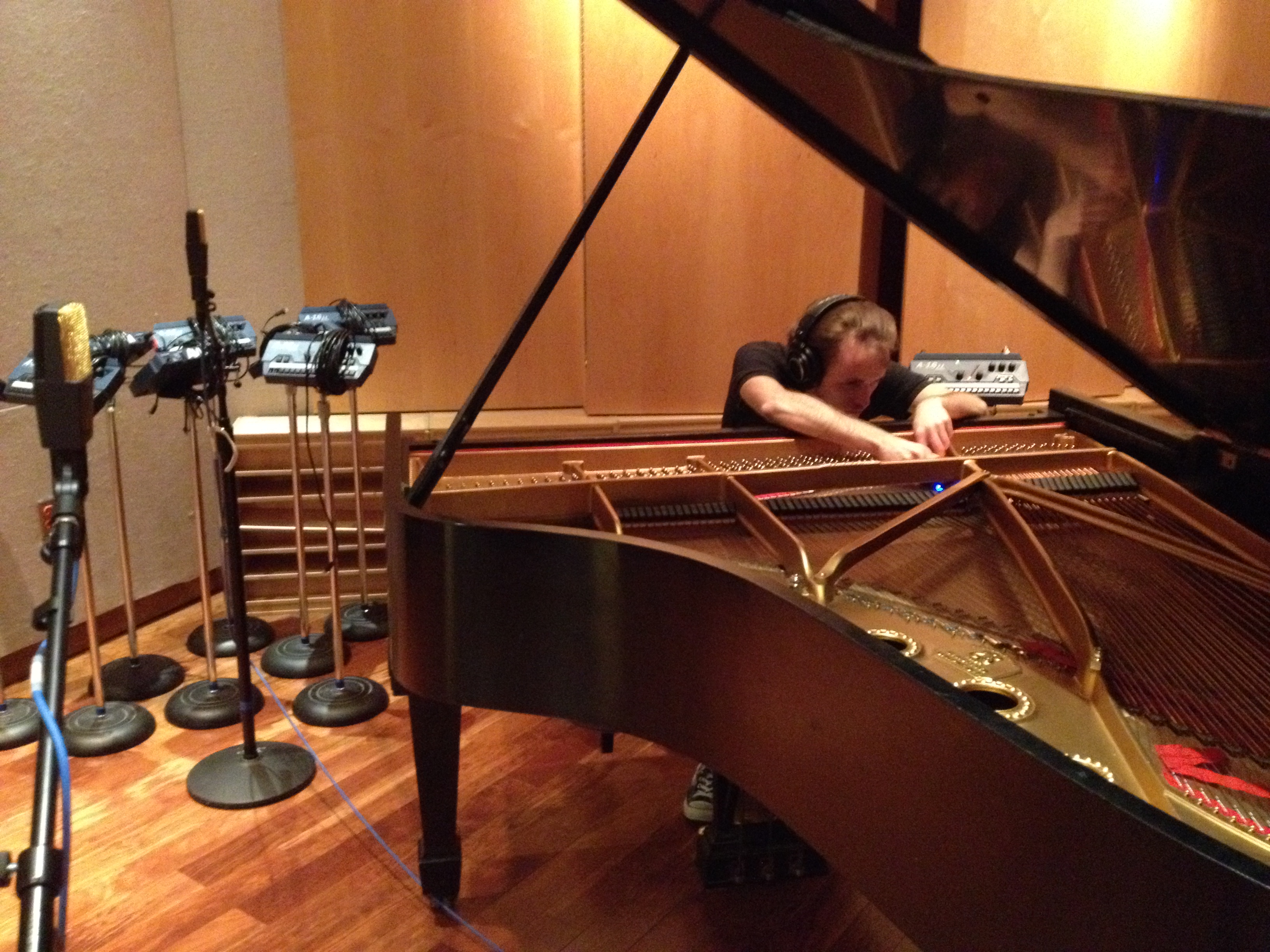
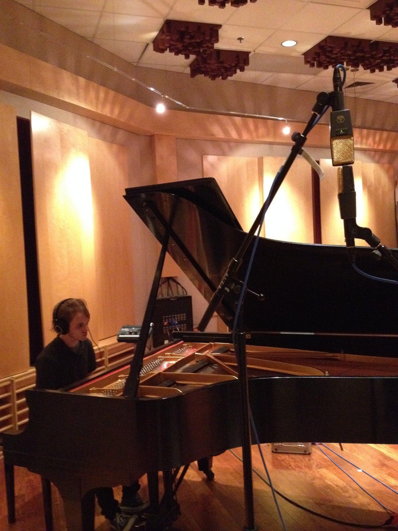
I made this with my friend Takumi Ogata last spring. Unfortunately, I couldn’t find any pictures of him playing bass.
e-bow action
I made this with my friend Takumi Ogata last spring. Unfortunately, I couldn’t find any pictures of him playing bass.
e-bow action
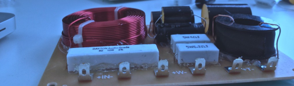
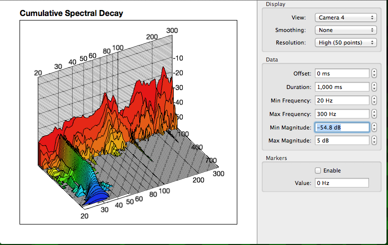
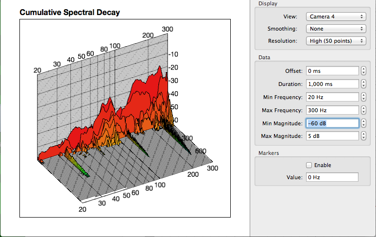
A port tube can extend the low-end response of a speaker beyond the lowest frequencies that can be produced by the woofer at an adequate volume. However, one of the drawbacks is that it takes time for the port tube resonance to die out. The best way to represent this is with a waterfall plot.
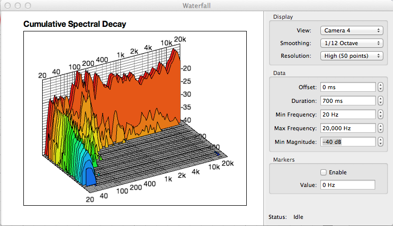
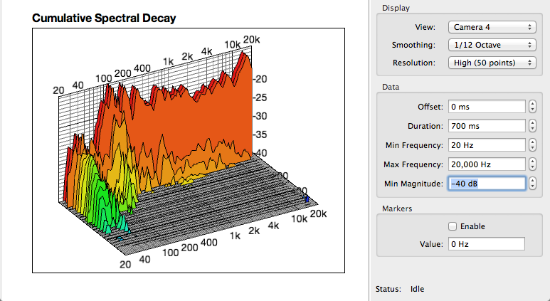
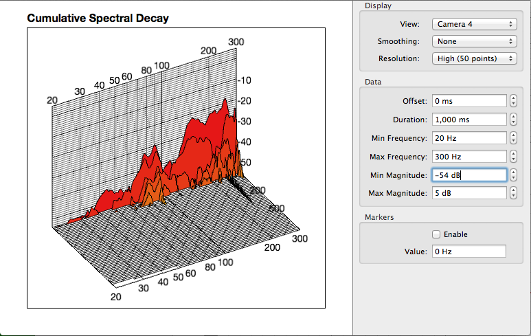
This shows the amplitude of all the frequencies decaying in time. The longest resonance is near the same frequency as the port tube. And when we plug the port tube with a towel…
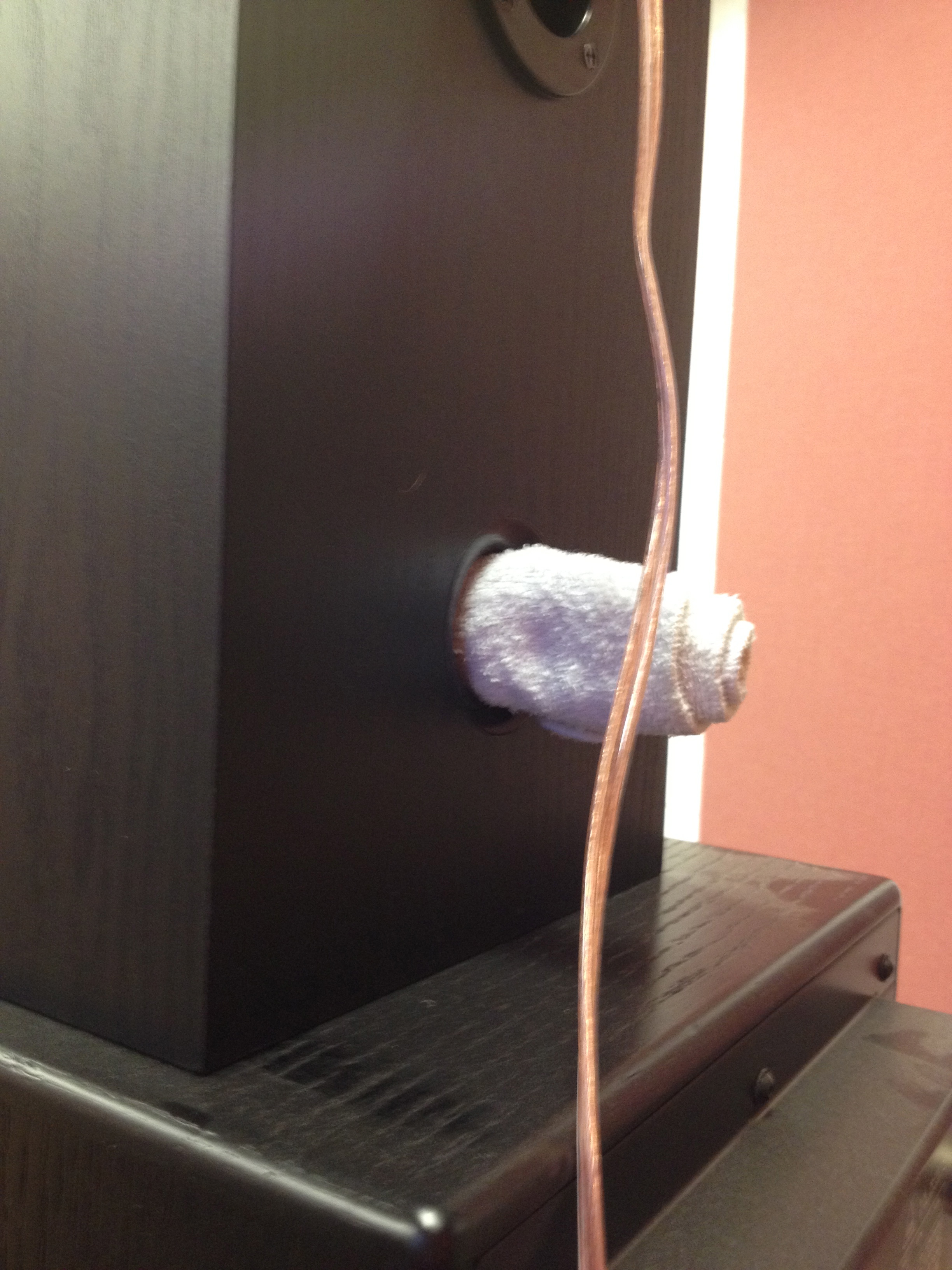
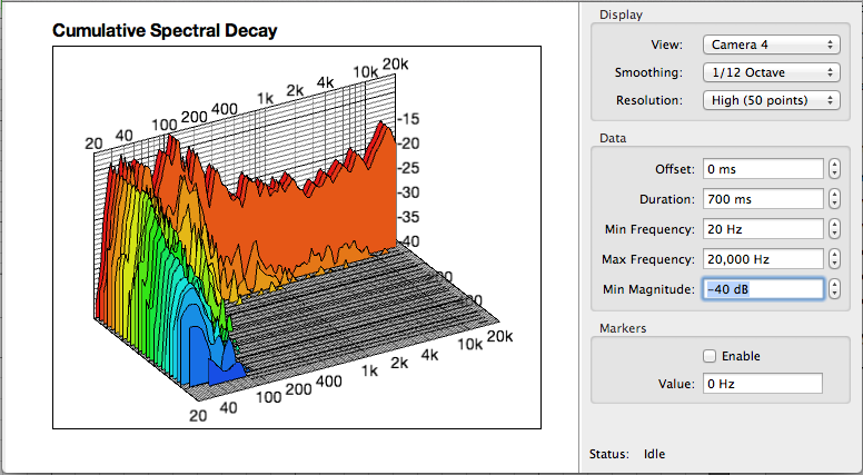
…. We can see that the resonance of the tube dies much more quickly.
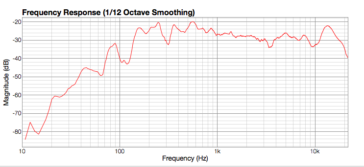
Subjectively, I want to hear more bass when I listen to the BR-1s, my speaker amplifier has a basic EQ, and the speakers sound more “flat” to me when I turn up the bass on the amp.
I find it interesting that what sounds “flat,” and subjectively pleasing to me is actually far from an ideal flat response.
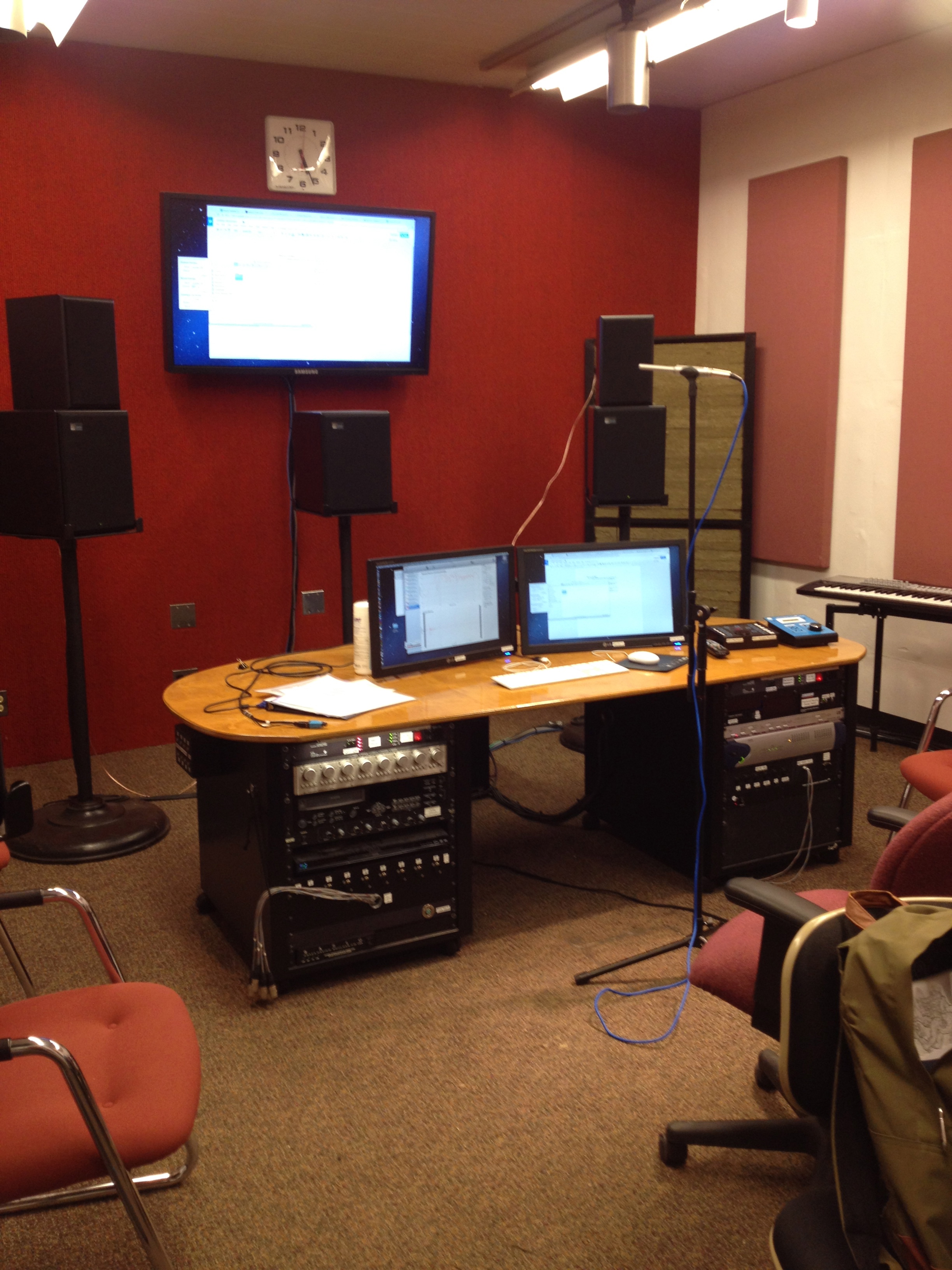
In order to better understand that data from the previous measurements, I also took some measurements at my apartment.
PORT NOT PLUGGED
PORT PLUGGED
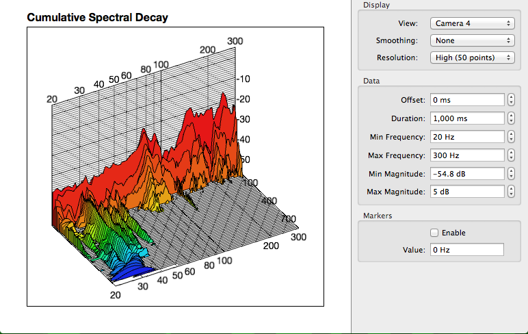
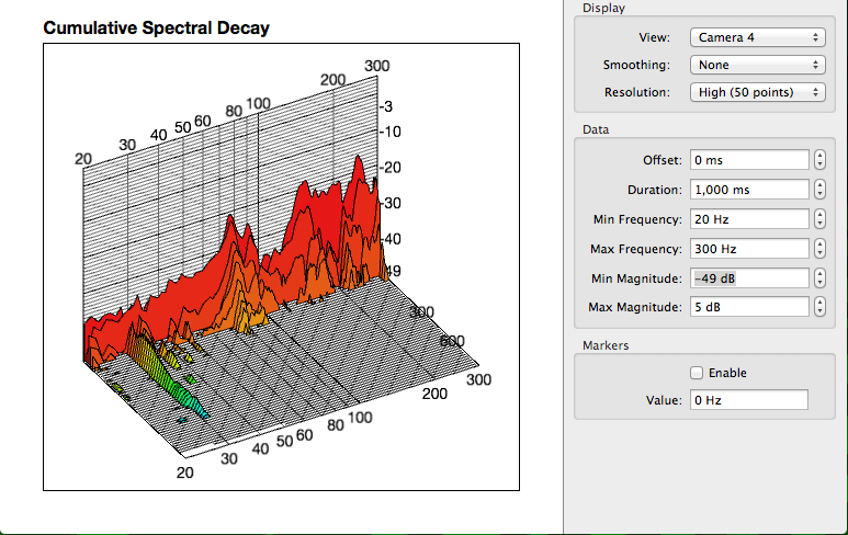
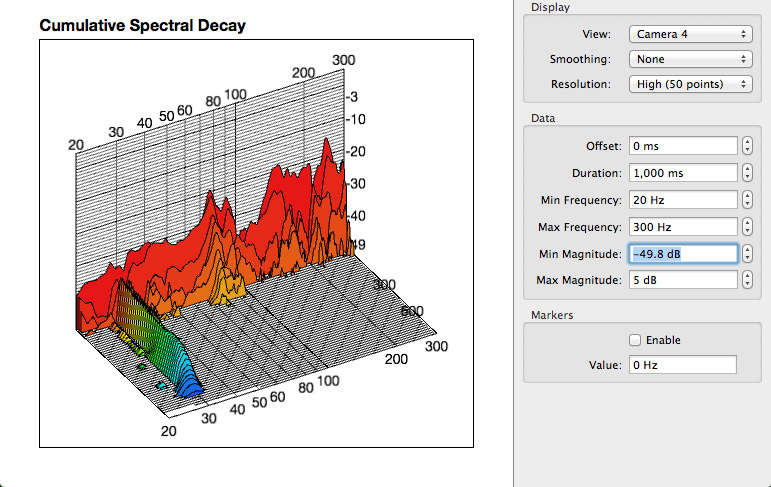
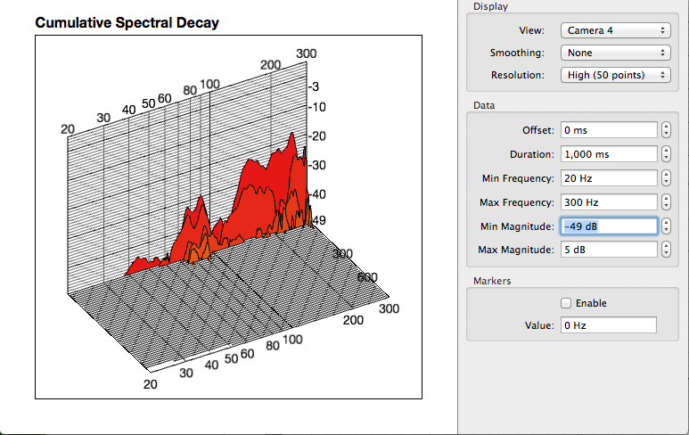
The graphs above show how the minimum value of the amplitude axis can greatly affect how the graph is interpreted. I tried to have the minimum value of the amplitude axis just slightly above the noise floor, which was at about -40dB.
I also took measurements at my apartment with my Presonus M7 condenser microphone.
The Dayton Audio measurement microphone was clearly a good choice as the Presonus microphone leaves out a lot of the bass information.
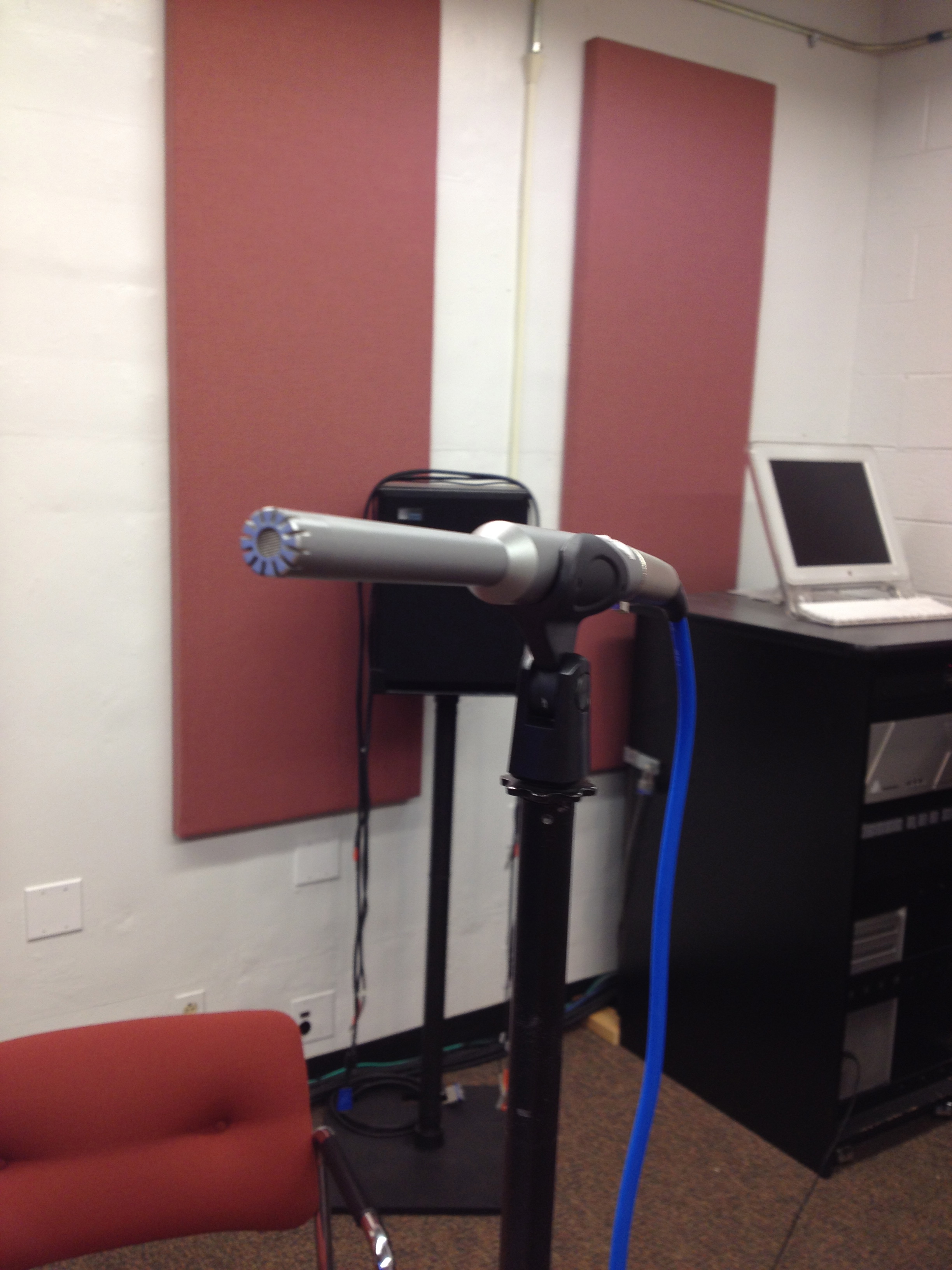
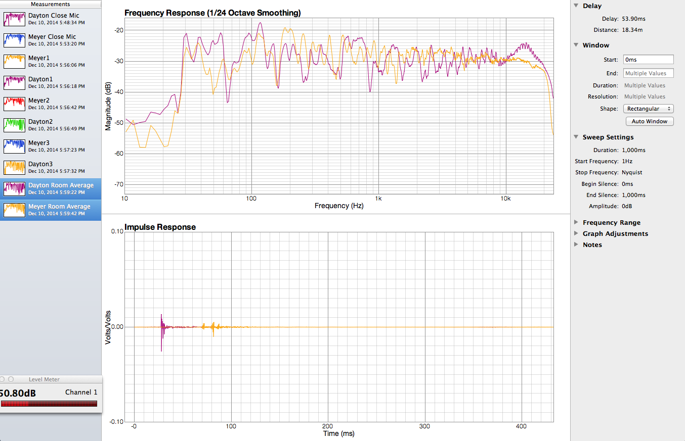
It is difficult to measure the frequency response of speakers because microphones do not have a flat frequency response, and the resonate frequencies of a room make some frequencies louder than others. However, if we keep these variables consistent, we can learn about the performance of a pair of speakers by comparing them with other monitors using the same room and the same microphone.
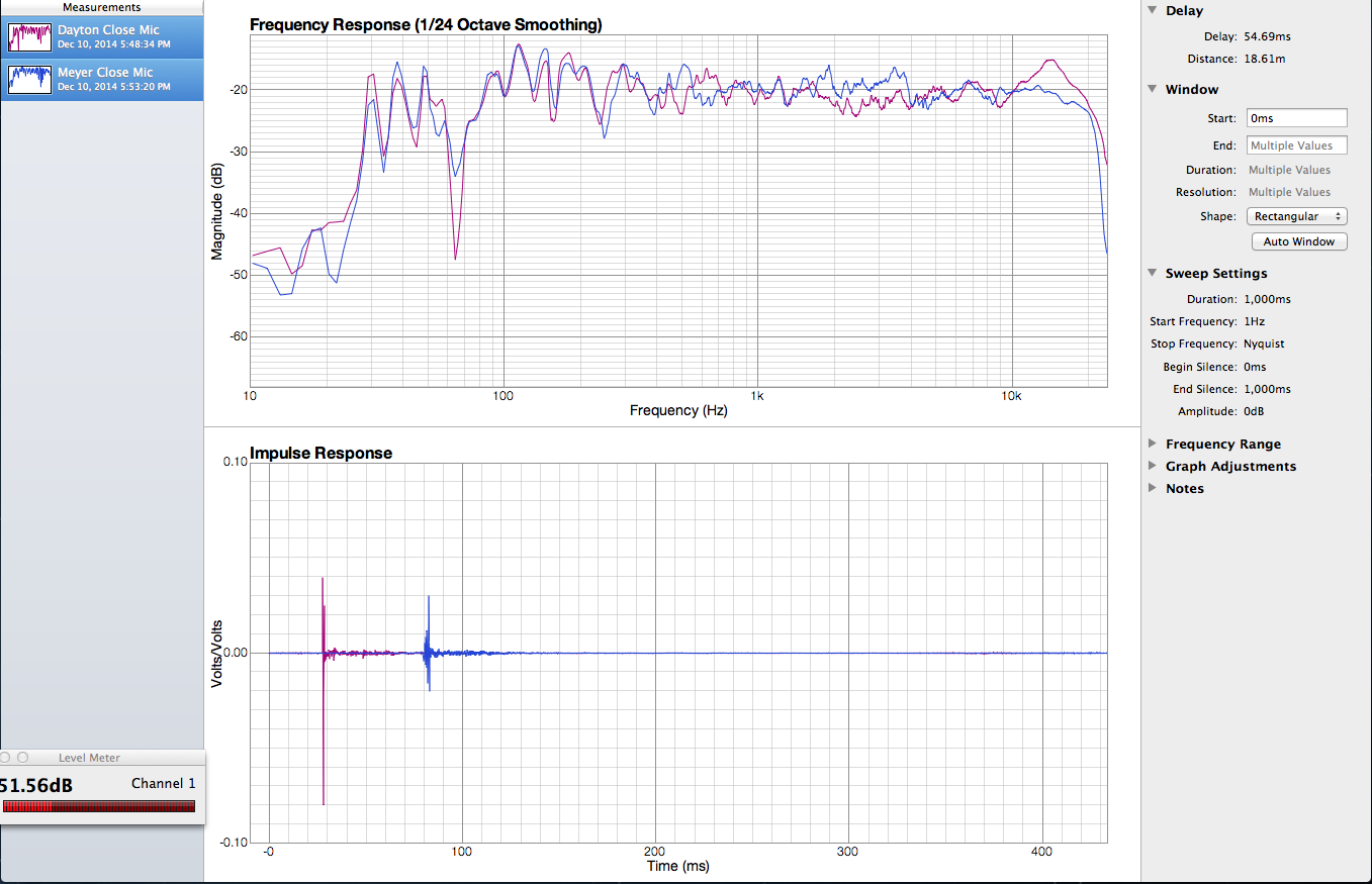
The image above shows the frequency response of my BR-1and a Meyer Sound speaker which I believe was an HD 1. These measurements were made with the program Fuzz Measure, the Dayton Audio EMM 6 microphone, and my Presonus Audiobox audio interface.
The most noticeable difference between the two speakers is the peak between 10kHz and 20kHz in the BR-1s and the deep trough between 60 and 70 Hz.
Here are the frequency response graphs for the individual drivers given in the manual.
.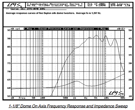
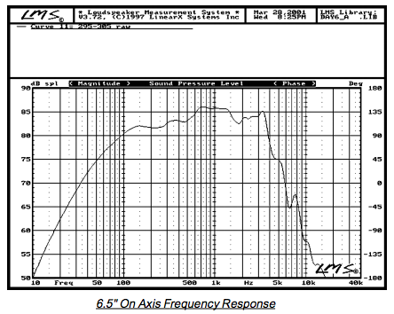
The stark differences suggest that my measurements were greatly influenced by the room modes. To try to compensate for this, I took measurements from many different locations around the room and averaged them.
The effects are noticeably reduced, and with a high enough sample size, could become negligible. However, it should also be noted that the resonant frequency of the port tube is 43 Hz– one of the peaks both graphs.

In the past few posts, I’ve been throwing a lot of words and equations at you, but I haven’t actually demonstrated that anything I’ve said is true. So here I’m going to demonstrate a few of the comb filtering concepts.
In my first comb filtering blog post I said:
“Therefore: f = (180°(2n+1)) / (360°*Δ) Now just plug in your delay time and values of n to find out which frequencies are canceled.
Let’s say your copied signal is delayed by .0005 seconds (aka half a millisecond). When n = 0,1,2,3,4,… f = 1000,3000,5000,7000,… respectively.”
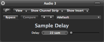
I want to show you that this really happens. In order to create this effect, I used an audio file (Little Lies by Fleetwood Mac) and a sample delay in my DAW, Logic 9. The track is sampled at 441000 samples per second, so if we want to find how many samples we need to delay to be equivalent to half a millisecond we observe:
(seconds/samples) * samples = seconds
1/44100 * samples = .0005
samples = .0005*44100 = 22 (approximately)
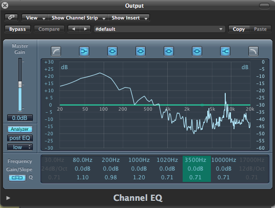
The effects are actually pretty apparent just by using the spectrum analyzer in Logic’s Channel EQ
No Comb Filter:
Comb Filter:
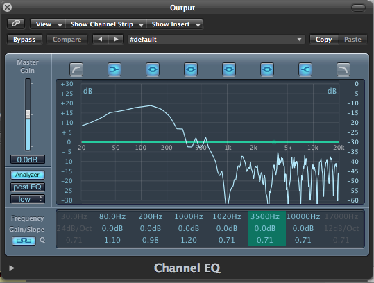
You can see that the frequencies that we predicted would be notched, 1000, 3000, 5000, 7000,… are indeed the frequencies that are notched. This difference between the two is clearly audible and I encourage you to try this on your own, as I am hesitant to upload copyrighted material.
From the first post, we know if we take two identical signals, delay one, and then sum the them, there will be frequency cancellation known as comb filtering. As abstract as that sounds, it actually happens in physical environments. If one of your speakers is farther from your ear than the other, two identical signals, one delayed, will reach your ears (the identical signals will be whatever is coming from the center of the stereo image, not the left and right). Another example might be the direct sound from the speakers, and the first reflection off of a desk or wall. Lastly, if you are recording an instrument using multiple microphones, an identical signal could reach the microphones at different times if they are spaced unevenly from the source.
What kinds of distances should we be concerned about? A foot? An inch? Here’s I’ll derive a formula for how distance corresponds to delay and frequency cancellation.
In the previous post, we found which frequencies are cancelled as a function of the delay:
f = [(2n+1)*180°] / [Δ*360°] where Δ is the time delay in seconds
We want to relate distance to delay. The units of speed of sound are feet/ second, so if we multiply (feet/second) by seconds, we get feet, the unit of distance. We also have a handy formula above that relates seconds to frequency. So here’s the math:
v * Δ = d (v feet per second, Δ seconds, d feet)
Δ = [(2n+1)*180°] / [f*360°] (f hertz — from the formula above)
v * [(2n+1)*180°] / [f*360°] = d (by substituting in Δ)
f = [(2n+1)*180°*v] / [d*360°] (frequency cancelled as a function of velocity and distance)
Because we solved out math problem in variables, we can choose the system of units we prefer. Because I’m from the United States, and most of the people who read this will probably be from the U.S., I’m going to use feet/inches.
v = 1100 ft/sec
Frequencies Cancelled:
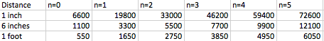
From the table, we can see that 1 inch is relatively harmless because the frequencies cancelled very quickly go beyond the range of human hearing. If we are setting up our microphones or speakers, we probably don’t need to worry about distances much smaller than an inch. This suggests that, rather than be concerned with minute delays from direct sound, we should be more concerned with reflections. Reflections will be the topic of the next post.
Hi! My name is Brian Kelley. Welcome to my blog!
This blog is where I will chronicle my adventures into the world of DIY audio. I have two main goals for the blog. I want this blog to be interesting to readers who already have a working knowledge of the subjects I will discuss. I will do this by including math and physics that could be interesting to readers with less formal backgrounds. However, I don’t want to write at a level that will exclude beginners. Although this is a blog about sound, I am passionate about the idea that language should never exclude anyone. I will try to use jargon minimally, and I will try to write as clearly and simply as possible- as I believe all writers should.
I’m currently assembling a pair of speakers that I’ll use for mixing. Later, I’ll work on positioning the speakers in my room, and acoustically treating the room. I’ll document that process in future posts, and I’ll also be publishing short articles on the physics that govern the decisions I make.
Stay tuned,
Brian
